Can graph mode improve problem-solving?

Polynomial factorisation & division

When students encounter a question that involves algebraic fractions, therefore dividing linear, quadratic and cubic expressions, there are a few different methods they can use. If they use an algebraic method, the quotient may either be a complete division or have a remainder. However, they can also use the graph mode of their calculator to visualise and draw the answer. We spoke to our mathematics expert, Simon May to uncover how graph mode can help students improve their problem solving skills. 

This approach can be helpful for several reasons. First, it allows students to double-check their work and make sure they have the correct answer. Second, it provides a systematic and structured way to approach the problem, even if the student is unsure of exactly how to solve it. By using this method, students can gain a better understanding of polynomials and improve their problem-solving skills.

Some interesting notes here:

• When you divide a quadratic by a linear expression, the resulting answer may be  linear, but not always..
• Dividing a cubic by a quadratic or linear expression, similarly may result in a linear or quadratic, but not always .
• If you divide polynomials of equal order, you probably get a an answer which when sketched, has vertical and horizontal or slant asymptotes.. This way, students can support whether the answer they got is correct or not.

Graphing the algebraic fraction and the  answer obtained from a division can provide valuable insight. Specifically, the roots of the polynomials  can give an idea as to what to expect from the  answer.

For example,

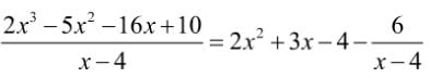
This quotient includes a remainder and so even before performing the division, students can see that the graph will differ from a division with no remainder.

The initial scales suggest an approximate cubic shape, which wouldn’t make sense, given the order of the polynomials. By changing the scales, students can now see a single vertical asymptote as expected at x=4 (when the denominator is zero).

This quotient includes a remainder and so even before performing the division, students can see that the graph will differ from a division with no remainder.

The initial scales suggest an approximate cubic shape, which wouldn’t make sense, given the order of the polynomials. By changing the scales, students can now see a single vertical asymptote as expected at x=4 (when the denominator is zero).

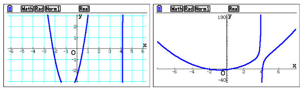
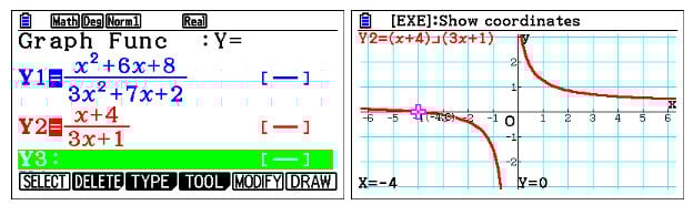
Consider:

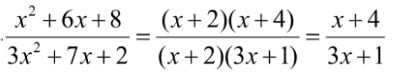
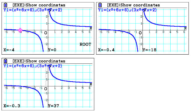
Sketching and analysing the initial fraction shows that  a root is found at x=-4, that implies the answer is going to be a fraction. It also implies the numerator is going to be x+4. Also, since there is a vertical asymptote, students can Trace and use the keypad arrows to move the cursor along the function and see the corresponding x and y values so that they can confirm when it’s moved from negative to positive along x axis, the y value changes from negative to positive as well. For example, if y=-18  when x=0.4 and y=37 when x=0.3, then it can be confirmed the denominator is zero when x is in between these two values.

What’s interesting here is if students can’t remember that they can factorise the top and bottom in such a question, they can just graph it, which can then help with the algebraic approach.

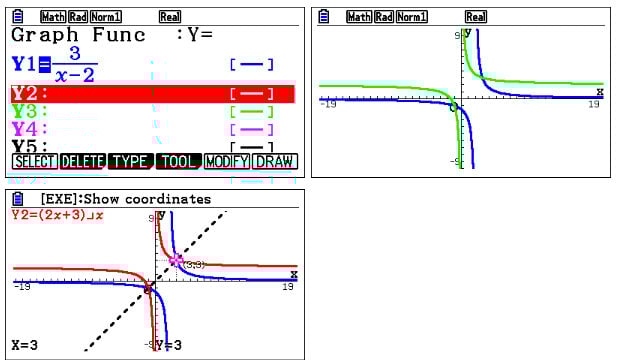
If students have two fractions and want to see whether one is a simplified version of the other and hence equivalent, they can simply graph both  and see whether they coincide which each other.

For algebraic fractions without remainders and therefore graphical asymptotes, the concept of factorisation can easily be introduced. Simon says: “With higher order polynomials, the difficulty of factorisation and understanding increases, but if you graph the question you are actually halfway there to solving it. So if you’re not sure how to proceed, just sketch it”. 

When a cubic function is drawn, it will have at least one x-intersect, and at most 3. “If there are only two visible roots in a cubic, it’s because one is probably a repeated root”, says Simon.

Consider:

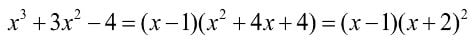
When sketched, one root is clear and the other appears repeated. Analysis revels this to be at x=-2. Therefore a student can now confidently attempt to divide through by (x+2) or even (x+2)² to find the other factors.

The calculating way to factorisation

Some students may struggle with factorisation . An alternative approach may be to  take a calculating route and use the wonderful “Table” function of the fx-CG50, where they can also plug some x values arbitrarily and see the corresponding y values. Then, they can see which (x,y) pairs have y=0 in them and thereby find the relevant roots and thereby the factors.

What’s even more helpful is, once a student decides the factors based on the roots, they can plot the division of the original function by the factor(s) to verify them visually. Students can even factorise the obtained quadratic further as well.

Factor theorem

This theorem states that if you put a value into a function and it equals zero, then that value subtracted from x is going to be a factor, which is the natural extension of what was just demonstrated.

To justify whether there are roots in a certain given range of a function, students can check whether the sign of the y value changes from positive to negative or vice versa in that range. This can be a very good place to start, especially using the Table mode.

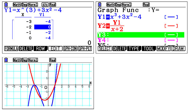
Take another example which has an even more complicated expression to factorise such as the one below.

One hack to find the factors is to check the numbers in the expression itself.

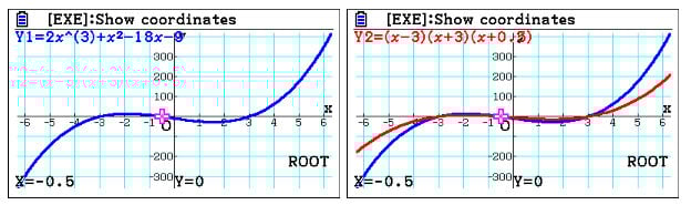
For example,  the constant is -9 and so the students can guess there has to be a “3” somewhere in the answer. Once the function is graphed, students can check whether the multiplication of the root values equals 9. Since it’s not in this case, it’s important to pay attention to the number at the beginning which in this case is “2”. When multiplied by the proper value, the multiplication of roots should give the required answer.

Composite functions

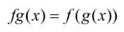
Sometimes students can get confused with composite functions, especially due to their notation. It’s important to have a clear idea of this notation so that students can use the calculator to support their answers. A composite function can be represented as   and when evaluating, there’s a shorthand way and a longhand way. 

Consider:

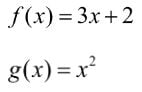
To find:

 In the shorthand way,  the inner function :

is evaluated  and that answer value is plugged into the outer function f(x), to get the answer . In the longhand way, as:

The inner function is substituted into to give and then the total function is found.

Using the calculator can assist students understanding and speed calculations, so graphing or using Table is suggested.

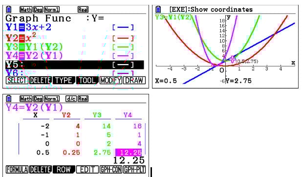
Simon: “You don’t want to interchange the inner and outer functions because that gives you two very different answers.” He also mentions that “If you’re unsure whether you have done it correctly, just stick some values in it and see.”

Range, Domain what are those?

A good question for students in an exam can be to find the range or the domain of a function. 

• Range is all possible values for Y
• Domain is all possible values for X

When the students plot on a graph, they can easily see the range and domain of a function. It’s worth noting that when you have horizontal asymptotes or vertical asymptotes extra care should betaken..

Inverse of a function

Inverse is basically undoing whatever you previously did to a function. For example, if you have a function to square x, the inverse of that square function is square root of x.

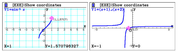
If a student is not sure where to start when finding the inverse of a function, it’s very easy to use the `Sketch` and then `Inverse` options to graph the inverse. This way the student can see the function and its inverse visually on the same graph.

By analysing these, a student could come up with the values for the answer with the help of the asymptotes. Here, it can be made even easier by drawing straight lines such as if needed.

About a function and its inverse, Simon says: “They are reflections of each other across the  line y=xso why not sketch that as well..”

Book a training session!

Using the fx-CG50 calculator to graph a mathematical function can make a world of difference. Mathematics Expert Simon stresses the importance of knowing about the features of the handset that allows students to get on the right track. This is especially true if they have just the slightest idea of what they’re trying to solve. 

Would you like to dive into the world of the fx-CG50 graphic calculator and get the most out of it? Then sign up for our free skills training sessions.